In this article, I want to have a look at randomness and what we can learn from it. The effects of randomness can be explained best with simple examples, therefore let’s play heads or tails:

You have to stake 100$ and when tail appears, your stake will be doubled, so you will have 200$. When head appears, your stake will be divided by three, so you will end up with 33.33$. If you play the game with always starting with your 100$ stake, the game generates positive results, as the expected value of the game is (200$+33.33$)/2=116.67$. So rational people without loss-aversion would accept the game!

Now, you are told that you have to play the game several times, but with only one initial stake of 100$ and at the consecutive rounds you have to use the result from the previous game. Here is an example:
Round 1: Tail -> 100$ x 2 = 200$
Round 2: Tail -> 200$ x 2 = 400$
Round 3: Head -> 400$ / 3 = 133$
Round 4: Tail -> 133$ x 2 = 266$
Round 5: Head -> 266$ / 3 = 88$

You might already have a hunch that the game has a negative expected value, and you are right. The expected value per round is 100$ x (2 x 1/3)^(1/2) = 81.65$. Only crazy people would accept this game.

But don’t draw a conclusions too fast. When dealing with random processes, as that is the case when tossing a coin, there can be a concatenation of positive or negative results. In this game you can just lose almost everything but you also have the chance to multiply your stake. Now, if you play 85 rounds of heads or tails, your chance of having more than the initial stake is at 2%. In other words: When playing the game 100 times (each game consists of 85 rounds, the coin will be tossed 50 x 85 times = 4250 times), you lose money in 98 games and win money in 2 game. It is even worse: in 90 games, you lose at least 99,84$ of your initial 100$. The game is still only suitable for crazy people, as the average expected value per game would be 4.30$.

But the more often you start playing the game, higher the chances for a long concatenation of positive results are. If you would have time to play the game 1 million times (85 million coin tosses), the average expected value per game would be 450,000$.
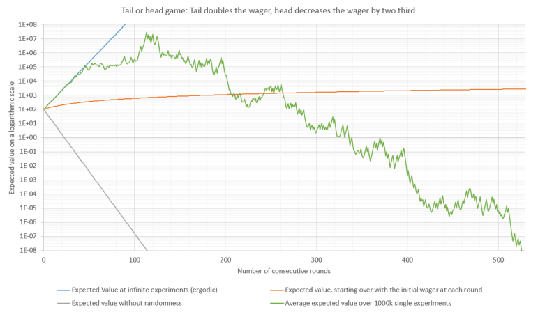
In the following graph 1, you see the the expected value (y-axis) in comparison to the number of consecutive rounds (x-axis). The orange line is with a constant stake of 100$ at each round, the grey line is without randomness, the blue line is with randomness and infinite repetition of the game and the green line is a real experiment with random numbers with one million executed games.

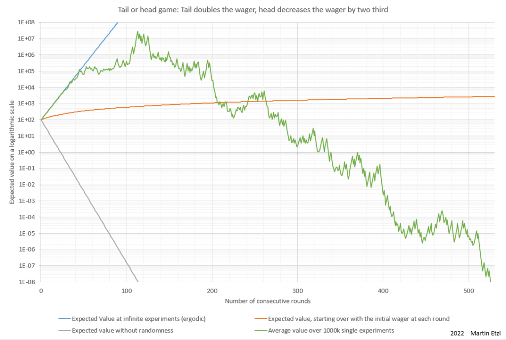
The expected value doesn’t need to be evaluated by experiments, but can also be calculated. In graph 2, there is a comparison between the average value over 1 million games (green line) and the average over 10,000 games (dark blue line). Additionaly, the expected value is calculated (purple and yellow line).

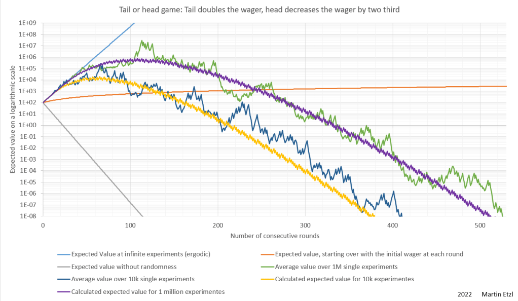
You can see that the more parallel games you play, the higher the expected value is. In graph 3 are several calculations with different numbers of parallel games.

The example of tossing a coin may be a simple example, but this rule might also be valid on more complex processes. One area of applying this rule could be in the stock market: Our limited ability to collect relevant information turns the stock market into a environment of low validity. We perceive this lack of information as randomness.

What can we learn from these random experiments?

In the tossing coin experiment we expect incredibly high losses. Nevertheless, it is possible to win a huge amount by playing the game multiple times with a certain number of consecutive rounds.

Even though you are playing a losing game, it is possible to turn it into a winning game by taking advantage of the concatenation of randomness.