This article describes an advancement of the logistic growth model, described in a previous article. The logistic growth model will be used for predicting future revenues and earnings of a company.

The model is especially suitable for high growth companies in order to give a clue of the value of the company. For companies at the beginning of the corporate-life-cycle, when costs and investment expenditure are high, revenues are low and earnings are negative, it is difficult to come up with an value. There, it is not feasible to measure value with P/E or EV/EBITDA ratios, even if they are forward looking.

The model incorporates many factors, such as:

• Market projections
  • How big will be the total addressable market
  • How fast will the market grow
  • Will there be a market decline some day
  • What will be the market share of the company
• Price effects
• Cost effects
  • COGS (cost of goods sold)
    • Experience effects
    • Economies of scale
  • Fixed costs
• Working capital
  • Including changes of working-capital-ratios over time
• Capital expenditure (capex)
  • Including investment lead times
• Basic corporate tax effects
  • Including loss carry forward
• Financing effects
  • Different interest rates at different debt levels
• Equity costs
• Inflation and it’s effects on debt, cash and working capital

As you can see, there are many input parameters and assumptions have to be made along the way. How many customers will there be, how often will they buy the product/service. In which markets will the company operate. Will there be a lot of competition? How will the price of the product develop? How will COGS be, will there be economies of scale and network effects? How efficient will the company use its capital for investments (will the company invest the money for mowing the lawn in front of the office every week, or will it use the money for improving the customer value of their product)?
With all these inputs, valuation becomes a highly uncertain endeavor.

I am still not sure, whether it is useful to do analysis with an advanced model. More complex models are more difficult to handle and often they do not deliver better results. Nevertheless, it is interesting to see the effects of different input parameters on the financial results.

In the following paragraphs, I will present the result of one scenario with fictive numbers for demonstration purpose. I will keep the descriptions brief, because in my point of view the graphs are the most interesting things.

Sales

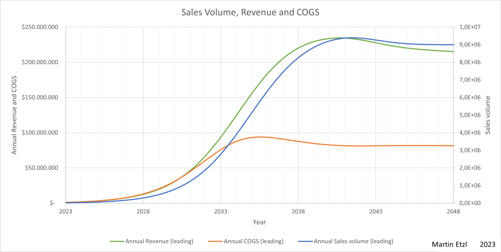
The financial model is starting with the assumption, that there is a logistic growth of sales volume. So, the financial model starts at a certain state with certain financial parameters (sales, cogs,…). Then, there is growth until a certain level of sales is reached. In graph 1, the development of sales volume, revenue and COGS over the years can be seen.

Following the corporate life cycle, this scenario starts with low revenue, followed by years of high growth until growth flattens and the company reaches a state of maturity.

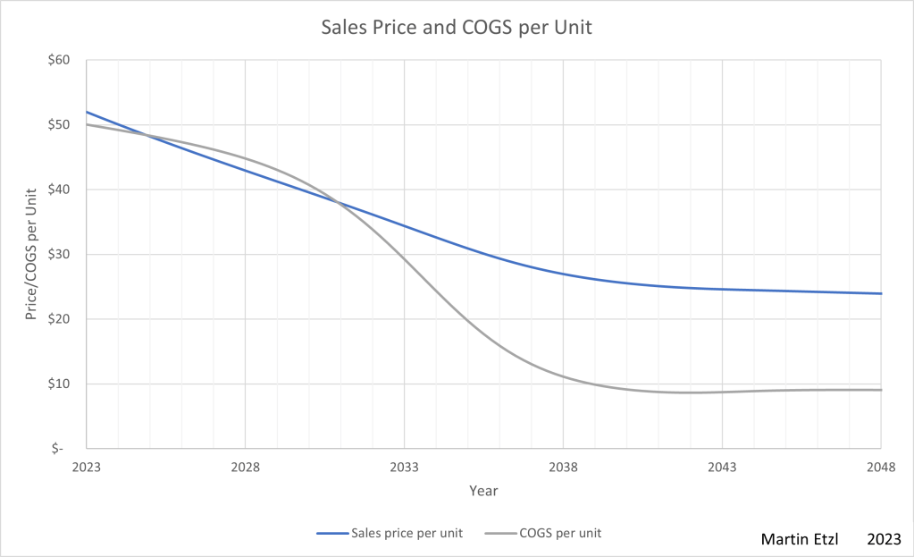
In graph 2, there are the development of sales price and COGS per unit over time. Experience effects and economies of scale have an effect on COGS. This means that costs will improve over time, because organizations learn, how to provide goods or services in a more efficient way. The sales price also decreases, as there might be more competition, or because it is economically more reasonable to decrease price in order to generate higher revenue.

Capex

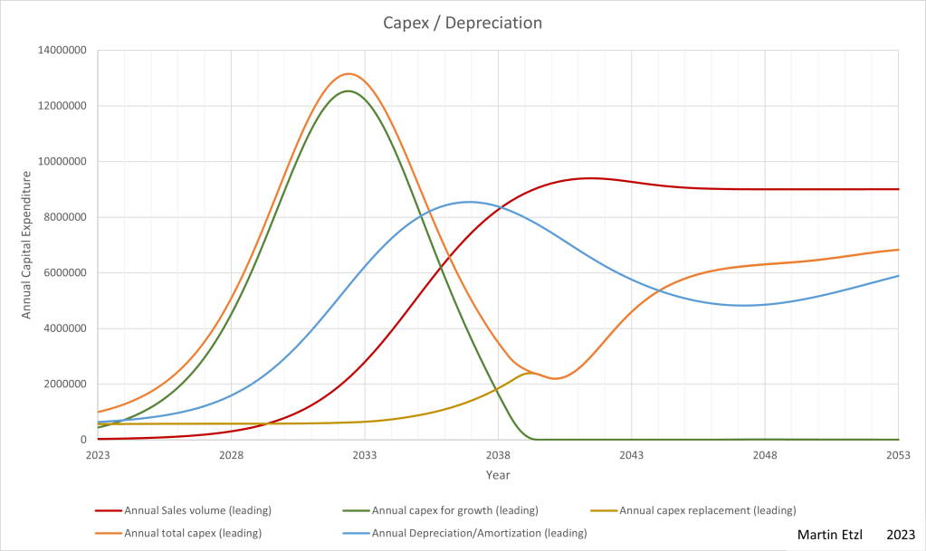
In order to grow, most companies have to invest a substantial amount of money in buildings, machinery, marketing, human resources, technology or other expenses. These investments have to be made in advance, which means that there is a lead time between the expense and its positive effect on revenue.

In graph 3, the capex over time can be seen. The capex is composed of two components, capex for growth and capex for replacement, as assets turns old and have to be replaced. The lead time between capex and revenue is clearly visible.

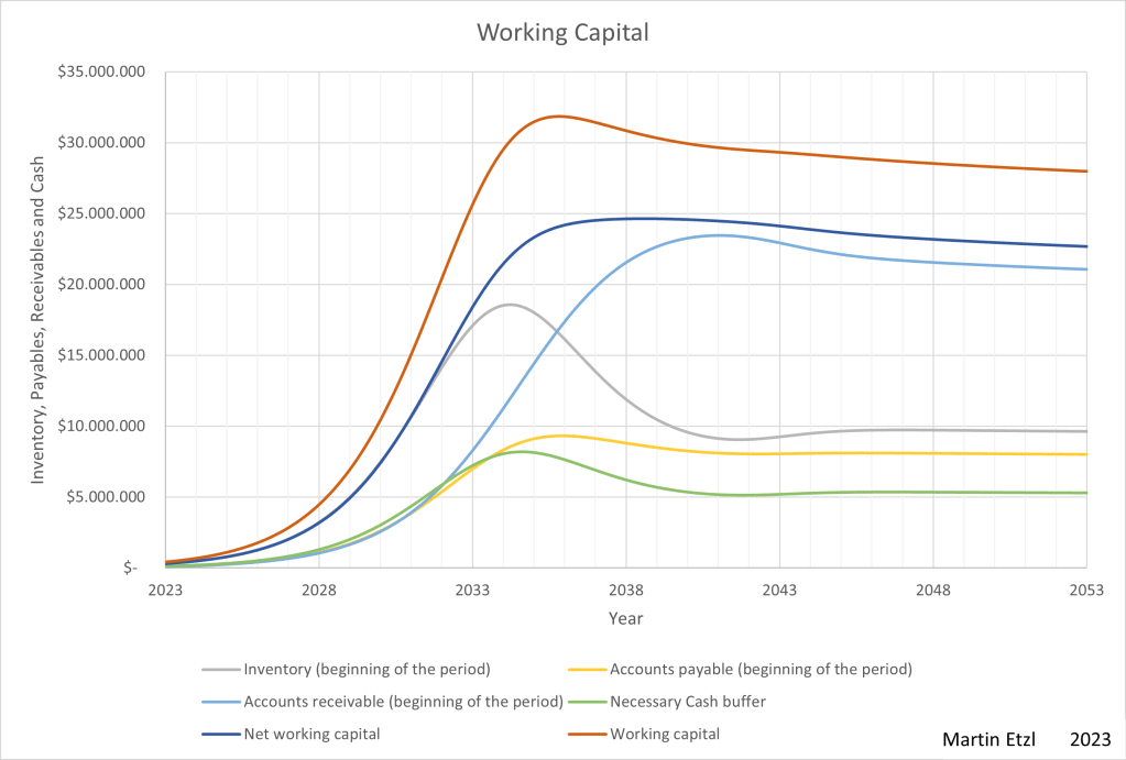
Working capital

Another influence on financials is working capital. Inventory, cash, accounts receivables are necessary burdens, a company has to deal with (in some cases, working capital can be negative). In graph 4, the increase in working capital can be seen.

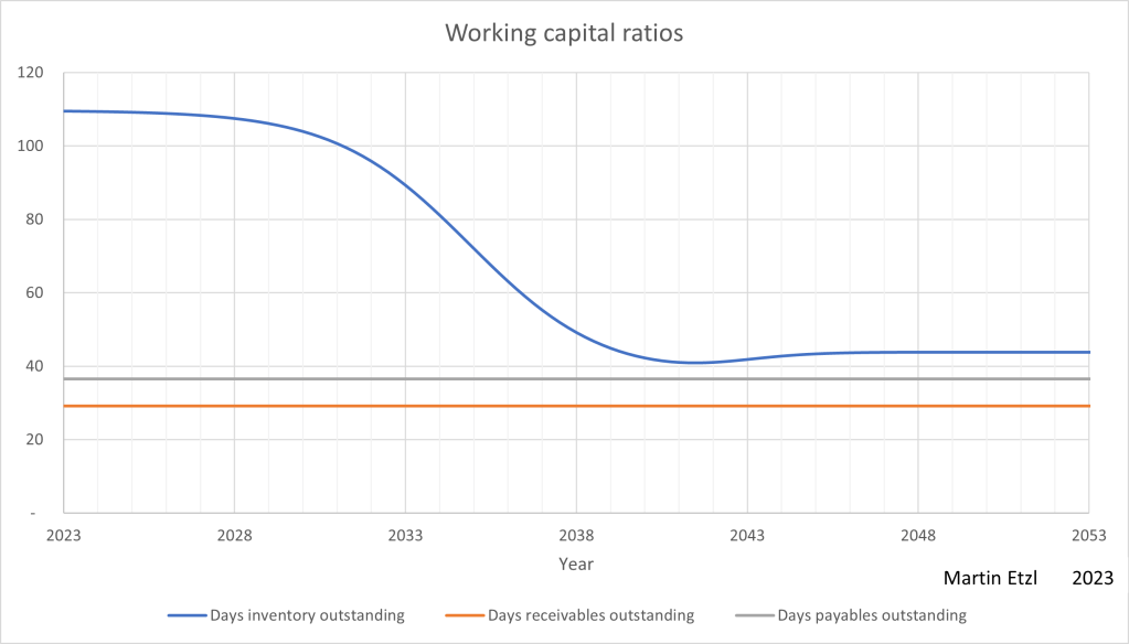
With an increasing revenue, the company will be able to manage its operations more efficiently, thus reducing inventory. This effect can be seen in graph 5, where the DIO (days inventory outstanding) changes over time.

Interest bearing debt

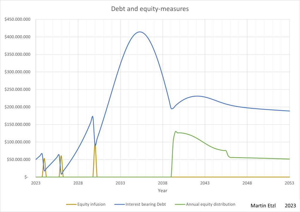
Another influence on the financial statements comes from interest bearing debt. In my model, the debt has an influence on the interest rate (the higher the net-debt/EBITDA ratio, the higher the interest rate).

In graph 6, the interest bearing debt can be seen. Several equity-infusions were made. By setting the input parameter to a target net-debt/EBITDA-ratio of 2, the model maintains this value from the year 2039 and instead of repaying debt, equity is being returned to the shareholder.

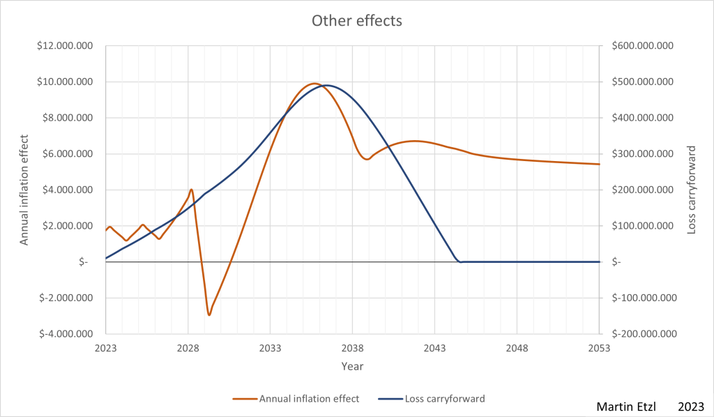
In graph 7, there are further effects, such as loss-carry-forward and inflation effects. The inflation effect occurs, when debts, payables, receivables and cash are being inflated away. In this scenario, debt and payables are bigger than receivables and cash most of the time. Thus, inflation has a positive effect.

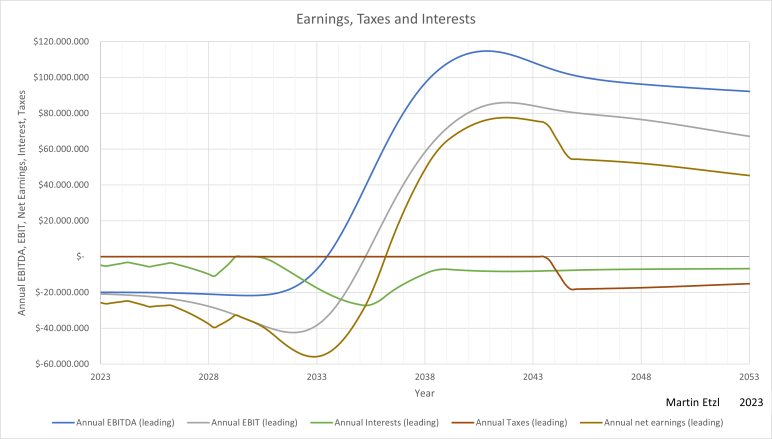
Earnings

Now, let’s look at the bottom line. In graph 8, different kinds of earnings can be seen. The influence of interests and taxes can clearly be seen on the net earnings.

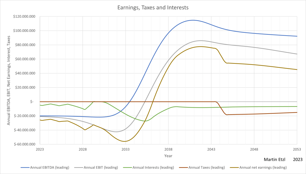
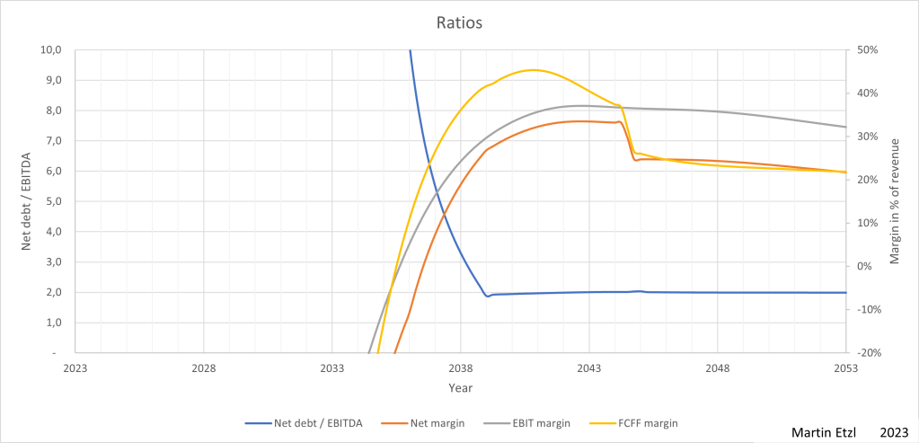
The ratios (earnings per revenue) can be seen in the following graph 9.

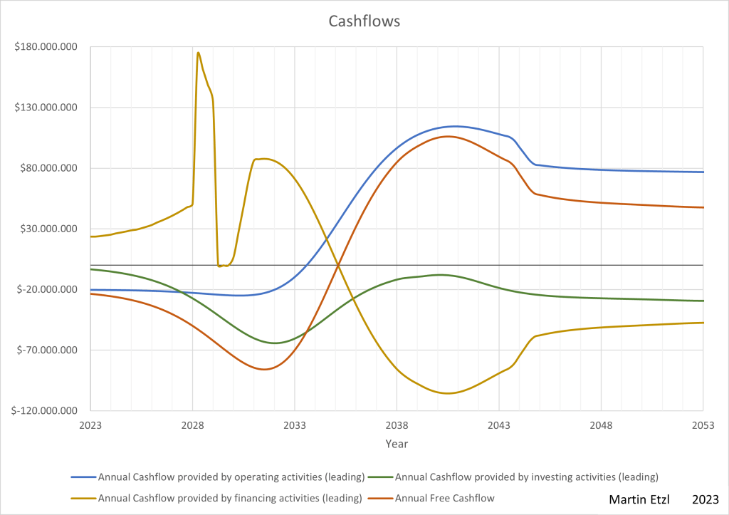
Cash flows

For investment decisions, Cashflows are more interesting than earnings, because cash flows tell investors, at which point cash is needed and at which point cash can be paid out. In the following graph 9, different cash flows can be seen:

• Cash flow from operating activities
• Cash flow from investing activities
• Cash flow from financing activities
• Free cash flow to firm
• Free cash flow to firm minus interests
• Free cash flow to equity
• Free cash flow to equity holders (the cash flow from/into the shareholders pocket)

In graph 10, the operating cash flow turns positive in 2033 and the free cash flow in 2035, due to the fact that the investing cash flow is high in the high growth state. Contrary to the free cash flow, there is the financing cash flow, which provides the money that is needed in the early years and returns the money to the creditors and shareholders, as the free cash flow turns positive.

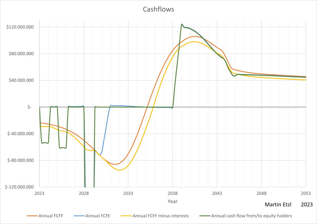
In graph 11, the differences of the different cash flows can be seen. While the FCFF grows more and more negative (mainly due to capex) in the beginning and turns positive in 2035, the FCFE has some negative cashflow years (due to equity infusion by e.g. issuing of shares) and in the year 2038 the company starts returning cash to the shareholder. (This FCFE is only possible, if the company finds creditors for the necessary debt)

Now, all values of the model are calculated precisely to the last decimal place. This, however, doesn’t fully answer the question about the value of the company. There are many parameters and each parameter could be different. This leads us to the next topic “simulation”

---

Simulation

In this case of financial analysis, the simulation will help to get a feeling of the range of valuation. By making the input parameters variables, the simulation tries out different settings of inputs on the model.

In my simulation model, I can set a range to each input parameter. For example, the total addressable market will be between 10M and 200M units per year. Then, the probability might not be distributed uniformly, therefore the model contains the option of choosing a beta distribution.

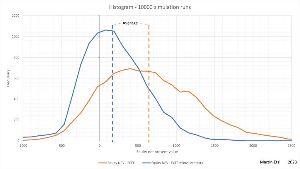
After some simulation runs, the result is a picture of wide variation of value (if you don’t set the parameters too tight). In graph 14, you can see a histogram of the distribution of the net present value of the equity.

The orange curve represents the discounted free cash flow to the equity shareholder and the blue curve represents the discounted free cash flows within the company. The difference in the two curves comes from the use of debt, which increases the equity value (Thanks god, we found someone paying the bills)

Conclusion

In order to do proper investing you have to make assumptions anyway. Why not putting these assumptions in a model and calculate a range of values. It makes me feel safer and more confident in valuation, when using the simulation and it is easier to find out whether it is worth investing in something.

Additionally, it is nice to see the development of financials visually. With scrutinizing income statements, balance sheets and cash flow statements, these numbers set an anchor in my brain, which provides a terribly wrong picture for future development of growth companies. When looking at the negative income in the last annual report, it is difficult to beliefe that there will be earnings in the future.

With the growth model and the visualization, it is easier to overcome the limitations of our brain.

---

For technically interested persons: The financial model is built up in excel and consists of over 600,000 calculated cells.