In my previous article, I described how an artificial intelligence would behave at picking stocks by looking at price data only. While the model performed slightly better than random, it gave me no reason to use this model as an advisor for my investments.

Meanwhile, after spending eight months in the valley-of-despair of A.I., I have finally created a model that can process fundamental data and was trained to predict stock price changes one year into the future. In this article, I will describe how my model works and how it performs.
(The model was trained on data from U.S. stocks covering the years 2000 to 2016 and tested from 2018 to 2023) (banks and insurers excluded) (as the model is 1 year forward-looking, I had to skip 2017, so that training and test data do not interfere)

How the model works

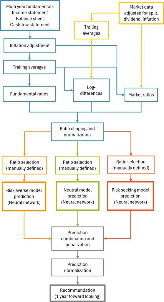
This framework, as shown in Graph 1, processes multi-year fundamental and market data adjusted for inflation and incorporates past developments through trailing averages and log-differences to generate selected key financial ratios. Using neural networks tailored to risk-averse, neutral, and risk-seeking strategies, it combines predictions to deliver one-year forward-looking investment recommendations.

The main model is risk-neutral, seeking a good trade-off between return and risk. A second model, trained for risk avoidance, not only reduced risk but also increased returns. The third model focuses primarily on maximizing returns with little regard for risk. It pushes the main model toward unknown and riskier terrain, helping it capture more opportunities. Overall, using three models increased the annual return of the recommendations by 2 percentage points.

The outcome is a daily ranking, where companies are assigned scores from 0 to 100. A score of 0 indicates a poor predicted future, while 100 indicates a strong positive outlook for the individual stock.

There are several key factors essential to the model’s predictive performance. I will explain some of them:

• Multi year fundamentals and fundamentals development
  • It is important to choose a suitable time period. Periods that are too short fail to smooth out fluctuations caused by business cycles, seasonality, or extraordinary events. On the other hand, periods that are too long make the model overly reliant on historical data and less responsive to recent changes.
• Ratio calculation
  • Widely known financial ratios cannot be directly used as inputs for neural networks. For example, the P/E ratio would introduce significant distortions and must be avoided.
• Ratio selection (the book “Quality of Earnings” by Thornton L. O’Glove was particularly helpful in selecting the right criteria)
• Past fundamental and market data must be adjusted for inflation to reflect the current value of money accurately (I used consumer price inflation)
• Heavy model regularization. Generalization of rules is more important than short term performance.
• During training, making the past and the future blurred

How to make the model learn the right things?

Training an artificial intelligence on financial data is like trying to tame a bull in a bullfighting arena — no matter what you want the model to do, it often results in the opposite outcome.

Data is the most influential factor in a model’s predictive performance. Boom-and-bust cycles need to be equally represented, along with both low- and high-interest rate periods and a sufficiently long history of fundamental data.

Additionally, the more a model is trained on specific details, the less adaptable it becomes for the future. For example, if a model learns from data from the late 1990s, a period dominated by the dotcom boom, it may conclude that investing in small companies with weak balance sheets and heavy losses generates the highest returns. I am quite certain that such a model would not perform well in the long run.

At one point, I tried adding industry sector information to the model, hoping it would identify sector trends. However, this led to undesirable predictions. Since the training data extended until 2022, the model favored pharmaceutical companies over other sectors—not because of any qualitative insight, but simply due to the pharma boom since 2020. That boom will not last forever. By adding this sector-specific data, the model became anchored to past trends and lost objectivity about the future, ultimately leading to under-performance.

Of course, there are long-term, global macroeconomic shifts that my model currently does not account for at all. This is a complex challenge that many persons struggle to address, and it is unlikely that A.I. will soon find an easy answer to it either.

The result

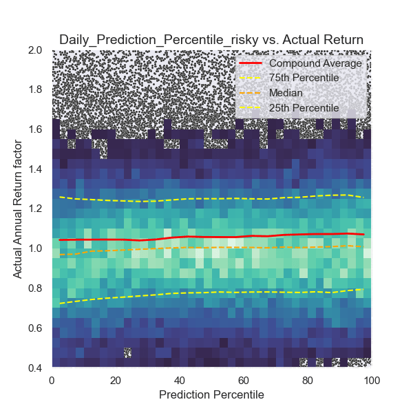
In Graph 2 below, you can see how the model behaves across its prediction range.

Each point on the graph represents a single company on a specific trading day. Since stock prices fluctuate daily, the model generates a new evaluation and prediction each day. When the density of data points is too high, the graph displays a color histogram instead, with brighter areas indicating higher density. Y-axis: Actual return of the stock. X-axis: Model prediction.
If the model functions correctly, there should be a clear correlation, where higher x-values correspond to higher y-values, indicating that stronger predictions lead to higher actual returns.

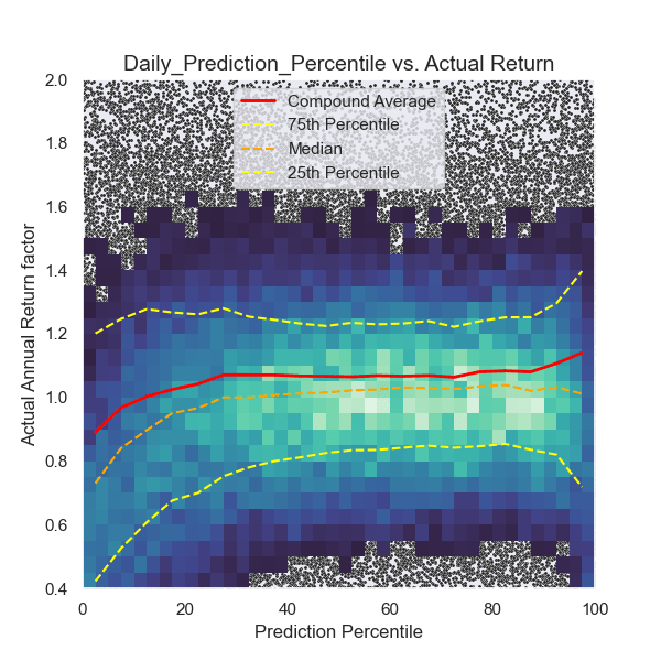
Even though volatility is high, the model successfully identifies patterns in the data to make future predictions.

• At prediction values below 40, a risk- and loss-avoidance pattern is clearly visible. The model effectively identifies stocks facing trouble, but it also misidentifies some opportunities that could have performed well. On average, returns in this range are lower than the market, and risk remains high.
• Between 40 and 80, losses are reduced, and risk is at its lowest. Returns in this range are approximately equal to the market.
• Above 80, risk increases again, but primarily in a favorable way, leading to a significant increase in returns compared to the market.

On average, the model understood its job surprisingly well.

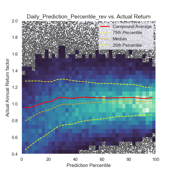
Below, in Graph 3, a different model is shown. This model was heavily penalized for losses, resulting in risk-averse behavior:

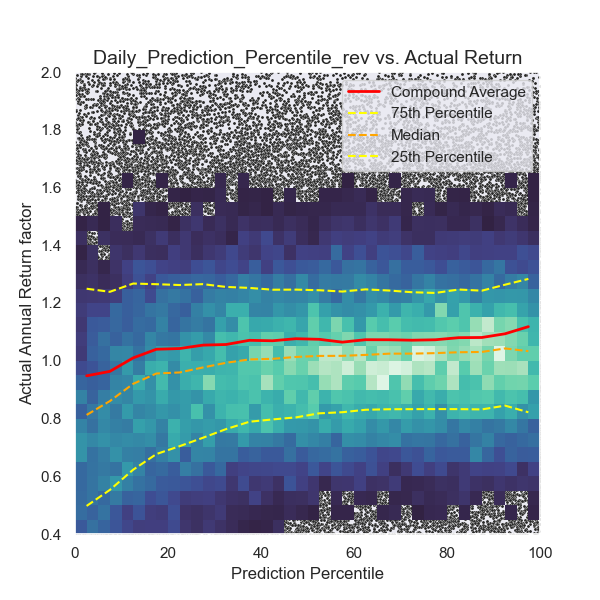
Low predictions correspond to high risk and frequent losses. High predictions show lower volatility and also yield higher returns.

Recommendation strategies

After receiving the model’s forecasts, I developed two investment strategies. (By “strategy,” I refer to the selection criteria for buy recommendations—whether to choose the top 5%, top 10%, or another approach.)

• Aggressive strategy
  • Optimized for compound return
• Conservative strategy
  • Optimized for lower risk

In order to have comparability of the models performance, I measure the models return (which is equal-weight-distributed) against the equal-weighted market.

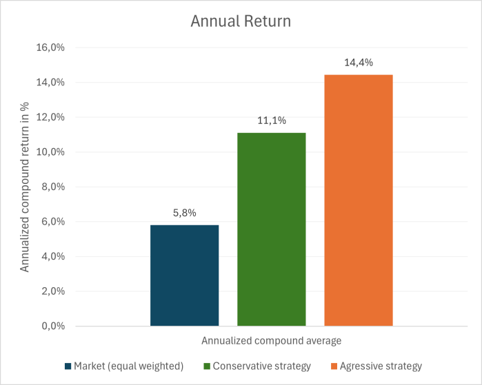
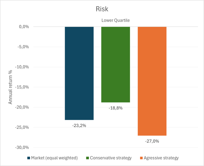
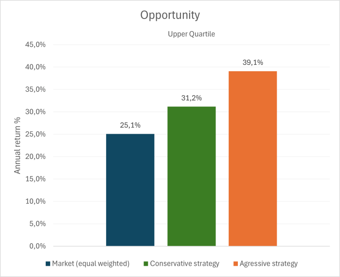
The aggressive strategy delivers the highest return, with an annual return of 14% — a 8 percentage point improvement over the equal-weighted market. However, this return comes at a cost, as the associated risk is higher (as shown in Graph 5).

The conservative strategy achieves an annual return of 11%, representing a 5 percentage point improvement over the market. Surprisingly, this strategy not only delivers strong returns but also significantly reduces risk compared to the market.

---

Conclusion

This research project demonstrates the impressive power of neural networks. With prepared financial input parameters, a neural network can see correlations between different financial ratios and future stock return. The relationships of high-dimensional and chronological financial data can be processed by neural networks in a way that would not be possible for human beings.

In the end, a model purely trained on fundamental and market data will never see how businesses, markets or countries change. It will not see the new cool product, the business is developing or a trend arising, nor will it see fraudulent balance sheets or inflated asset values.

However, what it does see to some extent is, if a company is on solid fundamental foundations and if the companies fundamentals are valued feasibly by the market.

With a significant avoidance of losses and an increase in return, the model is good enough as a risk-screening-model and I will use the model as a pre-selection-tool and a second opinion, when making my investment decisions.

---

Additional information for technically interested persons

Explanation of “Compound Average”: I created this to correctly consider parallel (diversified) and serial investment in companies. When investing in parallel, it is necessary to take the arithmetic average and when investing in serial, the geometric average must be used. I use a mix of the arithmetic and geometric average. (daily arithmetic + annually concatenated geometric + total arithmetic)

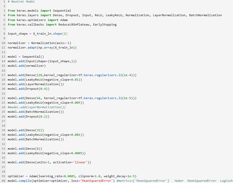
Even though using gigabytes of data for training, the final model fits on a floppy disk. The information consists of not more than a few thousand lines of code and a few thousand model parameters. Here is one model (based on Keras Tensorflow)

Making a neural network perform is not easy with noisy data. Below is an example of a failed attempt on making the risky model more aggressive and even riskier. It resulted in the neural network collapsing.

Making the risk averse model, being extreme risk averse resulted in skipping the slightest sign of volatility, but also in skipping many opportunities that would have made the model perform better.