The modern techniques of machine learning are a marvelous gift for processing tabular data and finding patterns, that can be used for predictions. Especially for high dimensional and noisy data where it is not so obvious to see patterns for humans, machines can see them. Not only the possibility to see these patterns, but also the speed of processing can be important. That makes machine learning ideal for doing fundamental analysis on public companies.

In my previous article Fundamental analysis with A.I., I was experimenting with stock market data to train models for recommending investments. I continued developing the model and want to show the results here.

The objective

By using pure financial data (stock price, balance sheet, income statement, cash-flow statement), the model should create a recommendation on stocks, ranked between 0 (not recommended for investment) and 100 (recommended for investment). To set clear limits of this experiment, there is no other information than fundamental data and stock price. For one prediction, the data from the past 5 years is taken into account in order to make a 1 year forward-looking prediction.

To back-test the effectiveness, a simulation of investing in the top recommendations is run and the average compound annual interest is calculated.

The model

The model consists of several parts:

1. Data import and data cleaning
2. Feature calculation and preparation
3. Embedding and clustering (K-means)
4. Neural Network models
5. Ensemble creation
6. Combination and penalization of predictions
7. Result: Recommendation

In total, 5000 models were trained on 6000 companies (including de-listed and bankrupt companies) with data from 2000 until 2017 and then tested, evaluated and compared during my research.

I used 48 different targets and different input parameter sets for training different models with different behavior. Some models are more conservative and try to avoid risk. Some models are more aggressive and try to catch opportunities, regardless of risk. Some models are trimmed for performing better in the long run and some models are made for the short run.

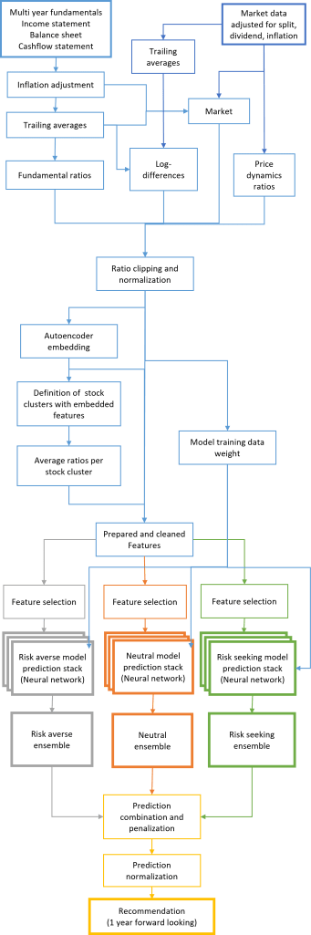
It would be too much content to describe 10,000 lines of Python code in this article, so I will keep the level of detail very coarse. In the graph 1 above, the schematic overview shows the flow of information through different modules of data preparation, ratio calculation, normalization, embedding, clustering, neural networks, ensemble creation, prediction mixing and finally the recommendation.

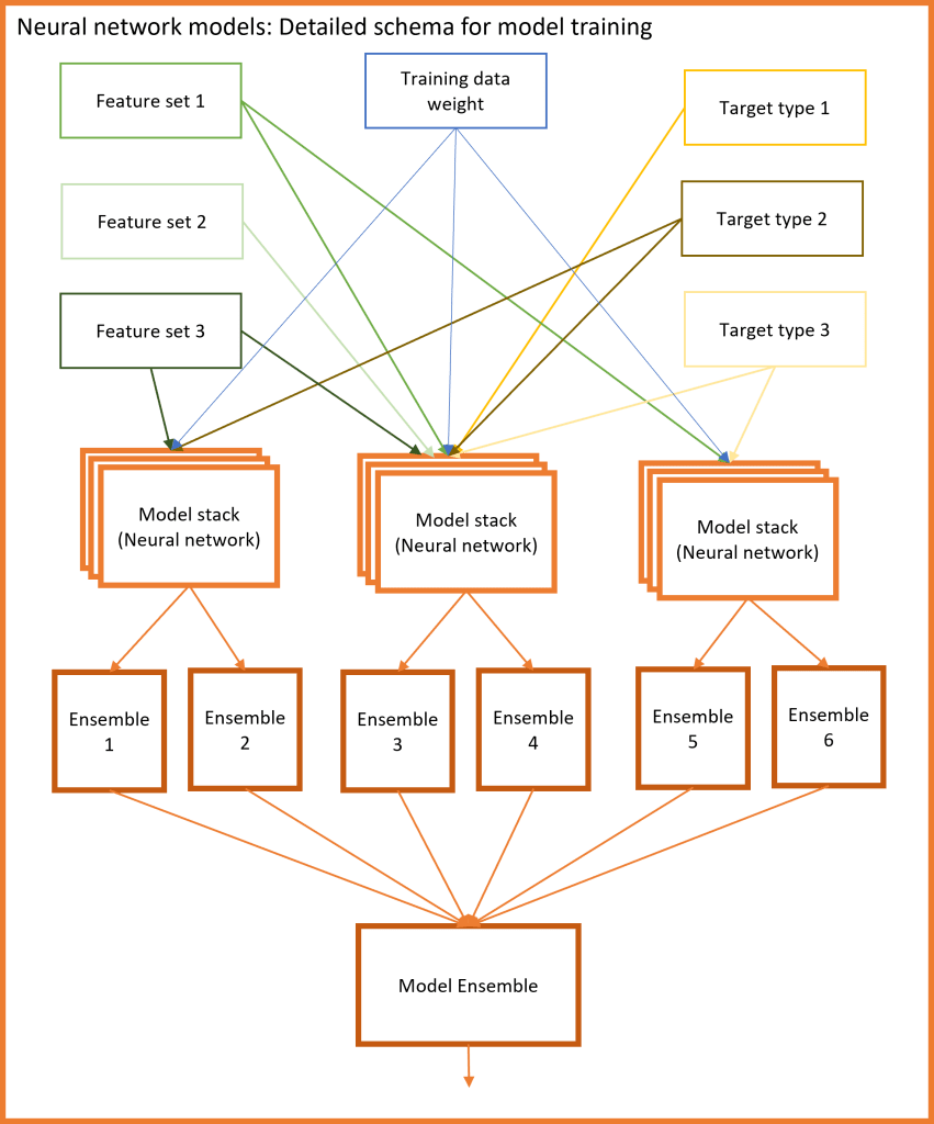
In graph 2 above, there is a more detailed schematic view of the neural network stacks themselves.
In total, 200 models are working together on my final version of the recommendation system. These models are combined through mathematical operations and rule-based combination to create the recommendation. The recommendation is always based on the latest data, and tries to look 1 year into the future.

Investment strategy

After getting the recommendations from the model, the next step is to turn recommendations into tangible results. I simulated to invest in the market from 2018 to 2025. For getting a clear evaluation of the model and the market itself, taxes and fees are excluded from the evaluation.

An important aspect of the investment strategy is diversification. By increasing diversification (also over different risk-classes), it is possible to increase return and decrease risk. (More about that in my article Managing randomness)

The result

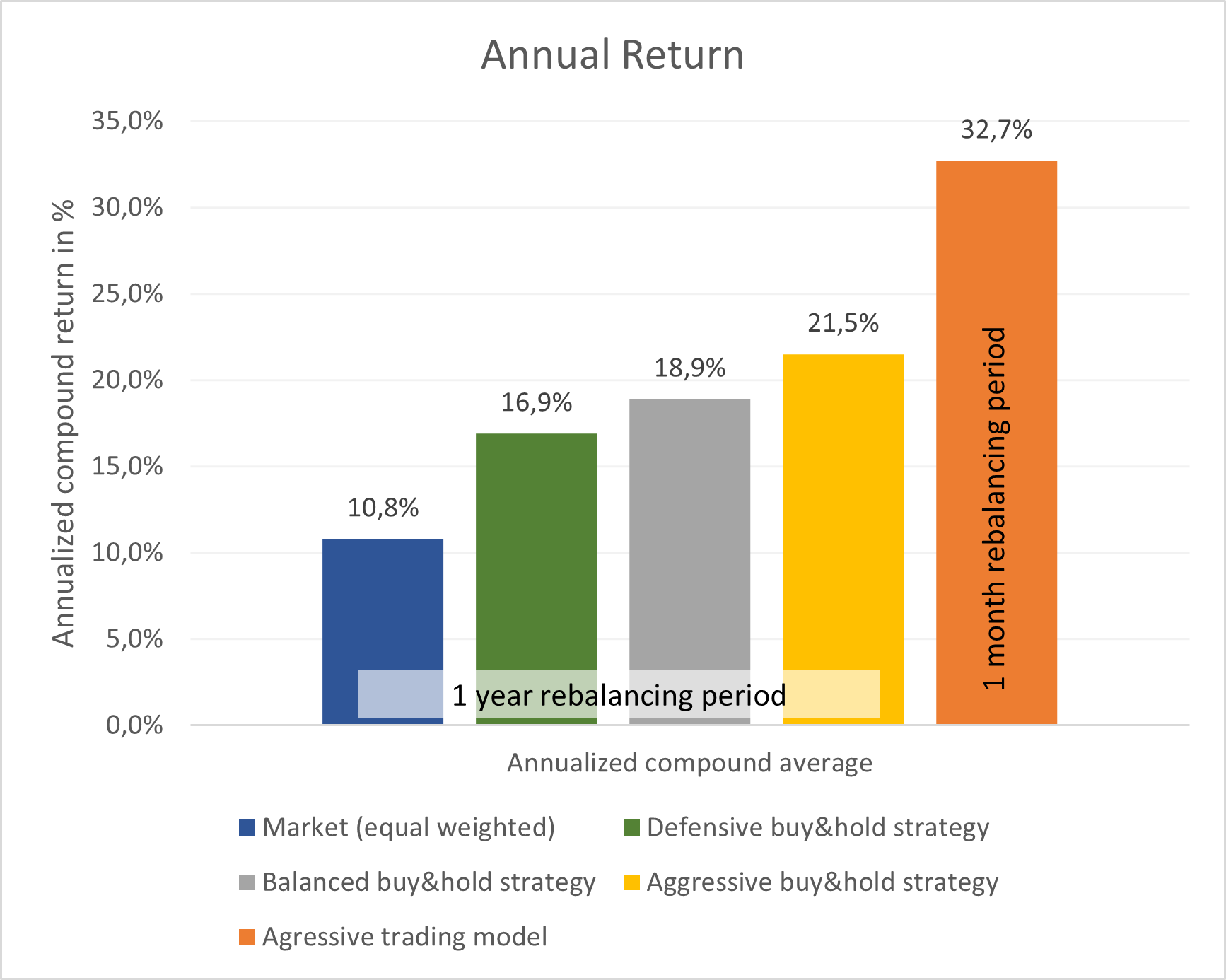
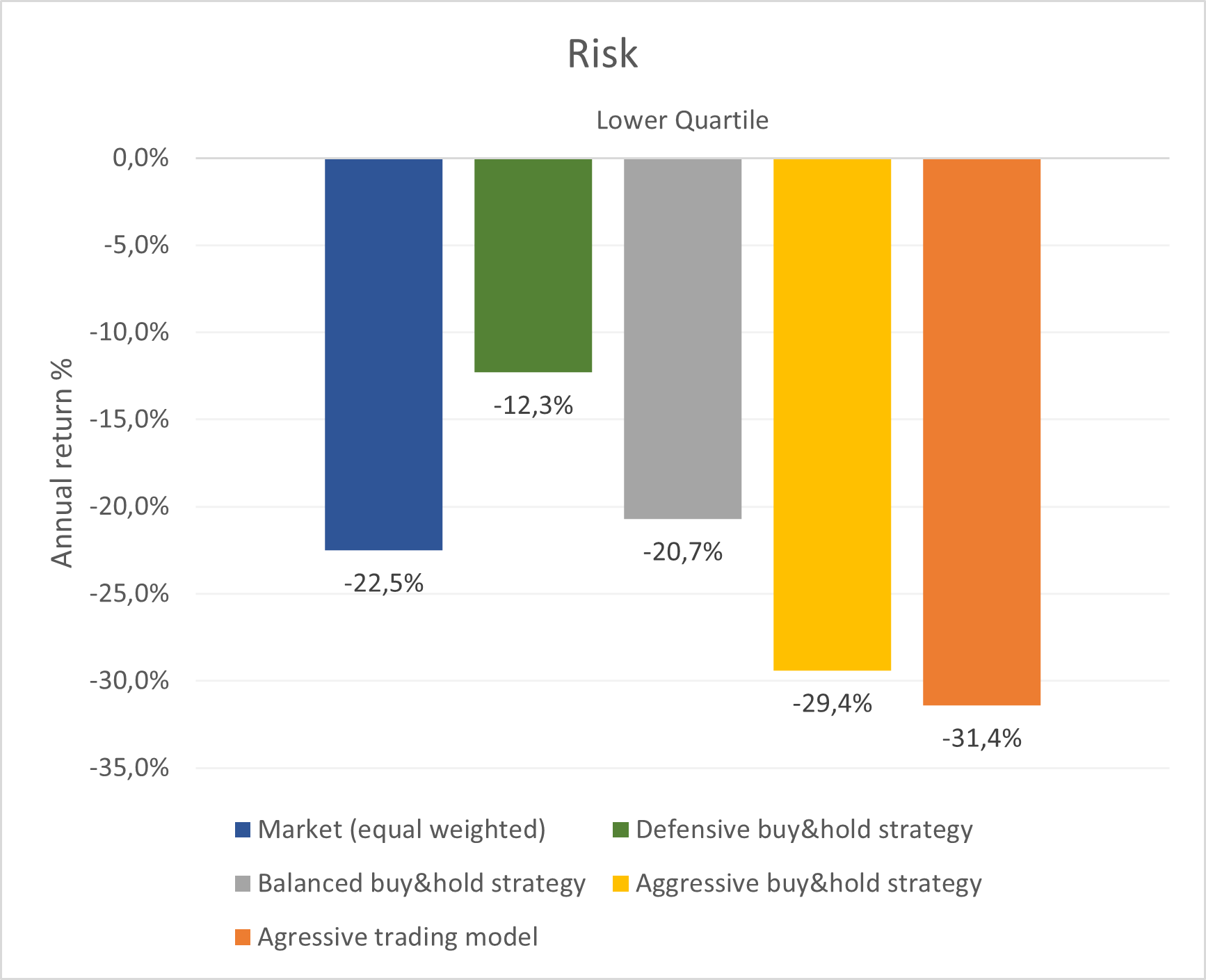
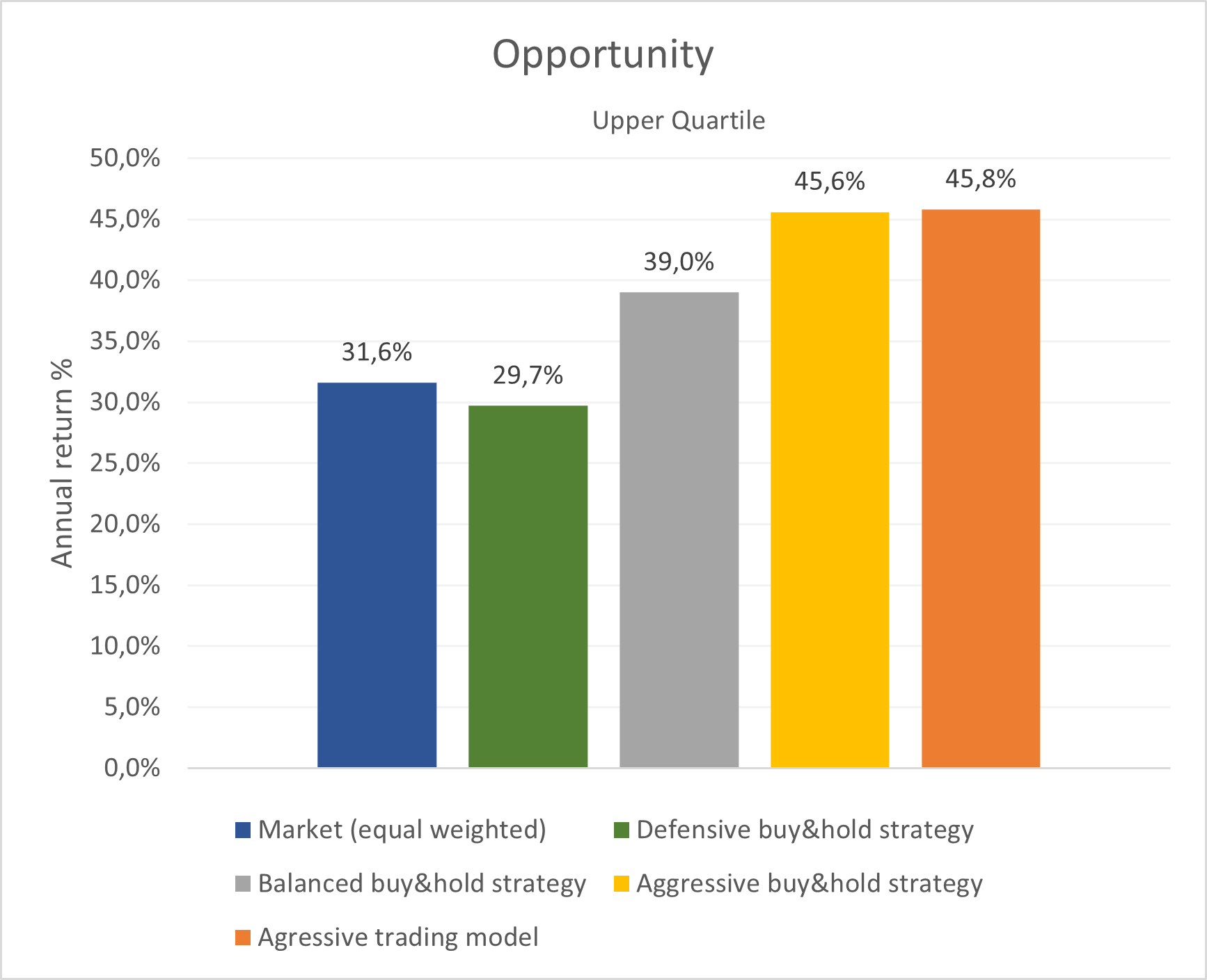
I wanted to create different models with different risk behaviors and investing horizons, ranging from defensive models with low risk up to aggressive models with high risk. The re-balancing period was set to 1 year ( and to 1 month for a more aggressive setting).

A special challenge was to my objective to create one model with very low risk. When cutting risk (this can be done easily by penalizing the model for losses and volatility), also the opportunities are cut. Thus, financial return is traded in for safety.
In order to anyway have a good return at low risk, it is something very difficult to achieve (everyone wants zero risk and high return. So the market reflects that human behavior and the high demand for low risk investments makes the price high and subsequently the possible future returns low)

However, if the models are trimmed well enough to detect overvalued or bad companies while not rejecting too many good and solid opportunities, it is possible to get higher returns at lower risk.
I was able to create a model that cuts risk in half and increases return by 50%.

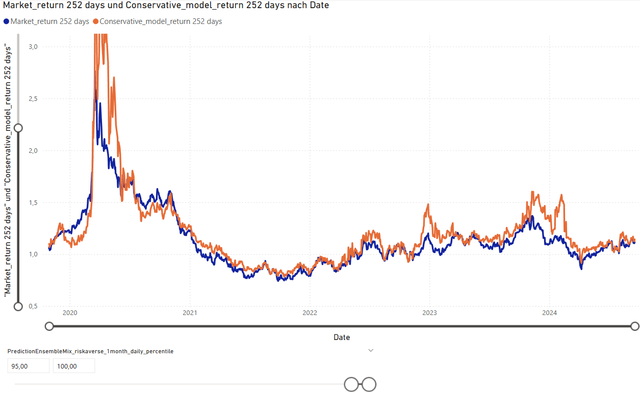
In the graphs 4, 5 and 6 below is a comparison of the different models and in graph. Graph 7 shows the 1-year forward looking return of the model per day, compared to the equal weighted market. The spike in 2020 shows the good investment opportunity after price drop in the corona-crisis early 2020.

Stability of the model under different conditions

While it is nice to have good recommendations that turn into high returns, more important is to have a model that is universally applicable and valid. The learned mechanisms and laws of the markets must be of real universal wisdom, that will be valid in the future as well. It would not make sense to train a model that succeeds on some trends or on some specific situations but fails in general. The model must not only be robust but also dexterous to handle different market conditions and different types of companies at different life-cycle stages (from high growth start-ups to cyclical companies to robust

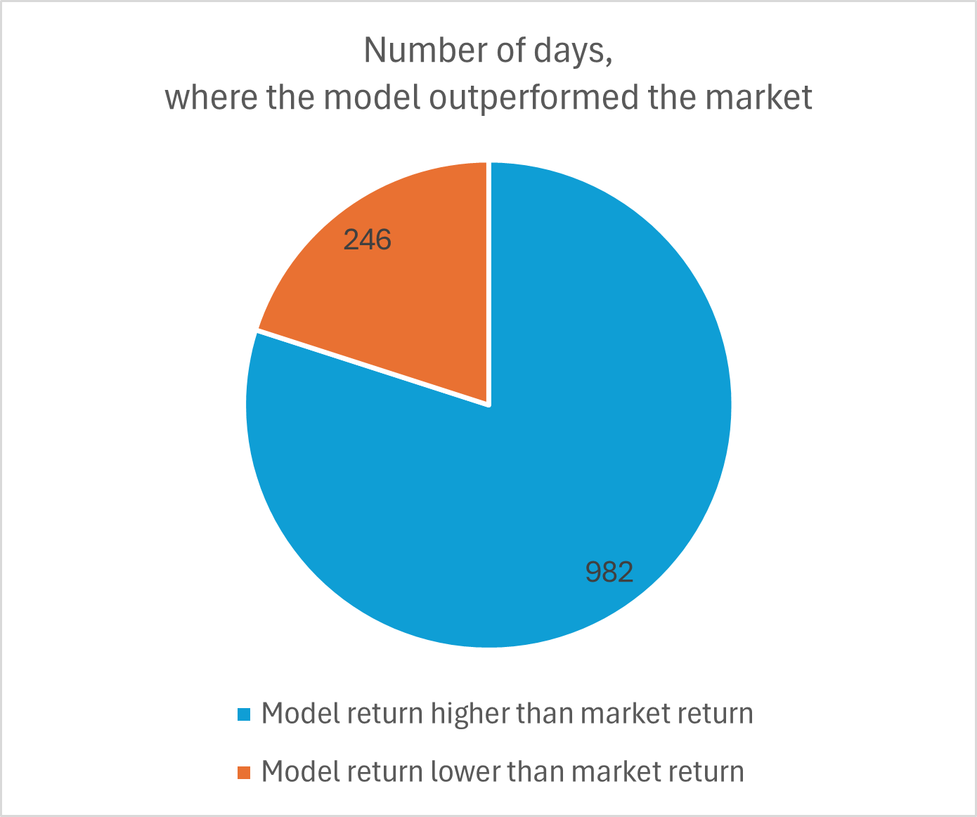
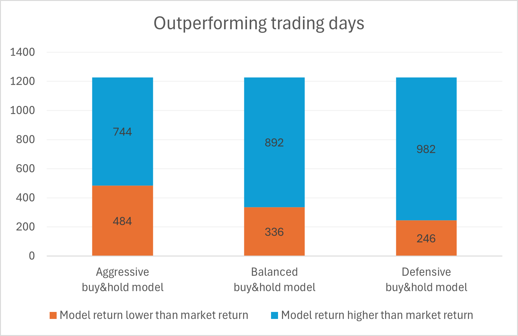
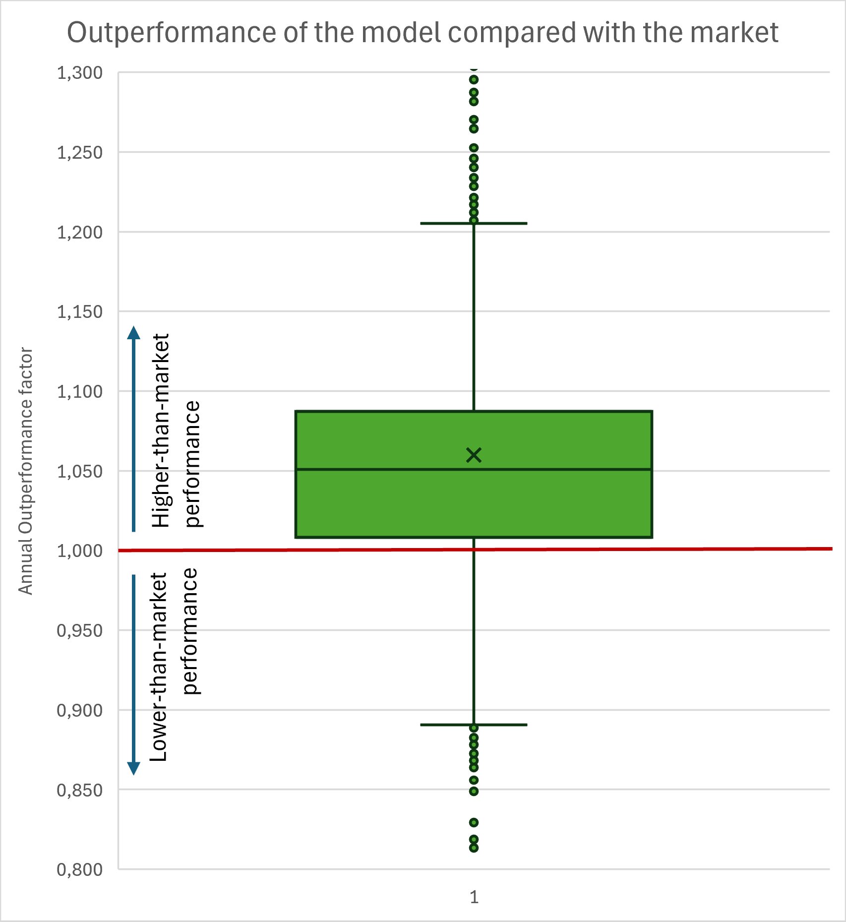
To measure the stability, I set my test period from 2019 to 2025 (I wish I had more data to cover a longer time period). On the following graph 7, I conducted an analysis on how many days, the model outperformed the market. This shows, that the model in general worked well not only on some occasions and outperforms the market on 80% of all days in the test period. Graph 8 shows the other models and graph 9 shows the frequency distribution of the market-outperformance-factor.

Disadvantages

For all these prediction models, there is a big unsolved issue (and maybe an unsolvable issue). The prediction is based on pure financial data from the past and thus the model behaves as if the future was the past. There is no such thing like speculation on future developments. The model can only see the revenue and the earnings of the past. It cannot see whether the business model of the company is still valid or on the edge of extinction.

To defend prediction models in general however, I want to state that to some extent, the rules of the past are the rules of the future (as in physics, the law of gravitation doesn’t change or in weather prediction, the rules of thermodynamics do not change, there are also laws that do not change in financial markets). And if a prediction system is able to extract the general rules rather than short trends, this can already make the difference between a performing and a non-performing model.

In my case, the prediction is based on a very limited time period (the last 25 years).

Conclusion

Through proper preparation of data, calculation of “machine-friendly” features, sound development of models and application of economic principles, it is possible, to create a stable model that reliably can decrease risk while increasing return.

In the end, the more philosophical question is, what influence will these models take on our world and how would they shape the financial markets. While the individual institutions with the best models will have a benefit over others and subsequently create higher earnings, there will be another side effect: the financial market will allocate resources faster and more efficient to the companies with the best prospects. Increasing financial resource allocation efficiency will lead to an increase in real world resource allocation efficiency, a decrease in loss and resource waste and subsequently a general increase in wealth and a decrease in poverty.

---

Additional information:

If pushed to the extreme, the model could behave much riskier, which also brought more returns in the test period between 2019 and 2025. I will not consider these high risk models as a valid option for an individual investor like me, because of the instability of the model and because of the high amount of work it would require, to execute this strategy.

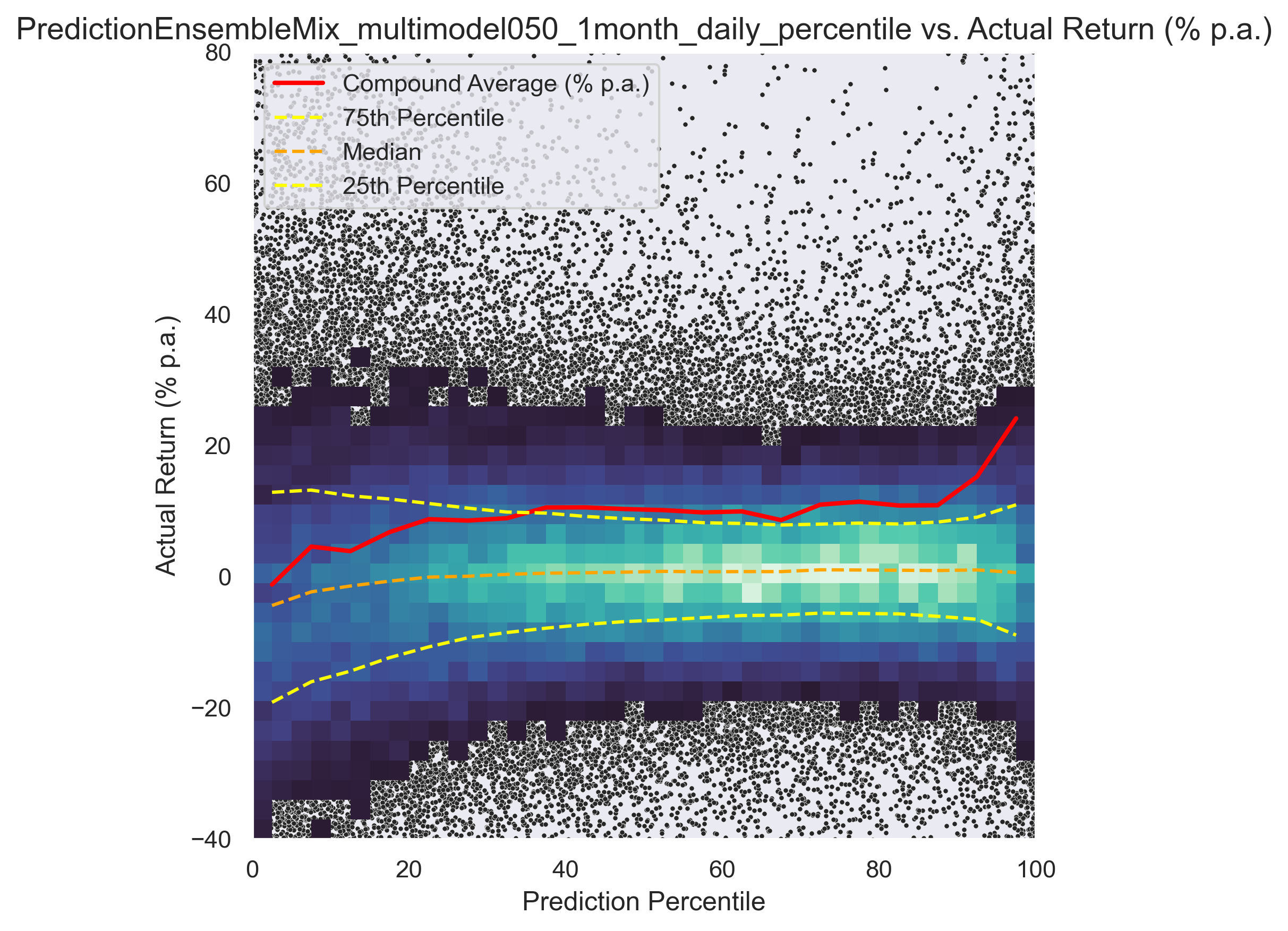
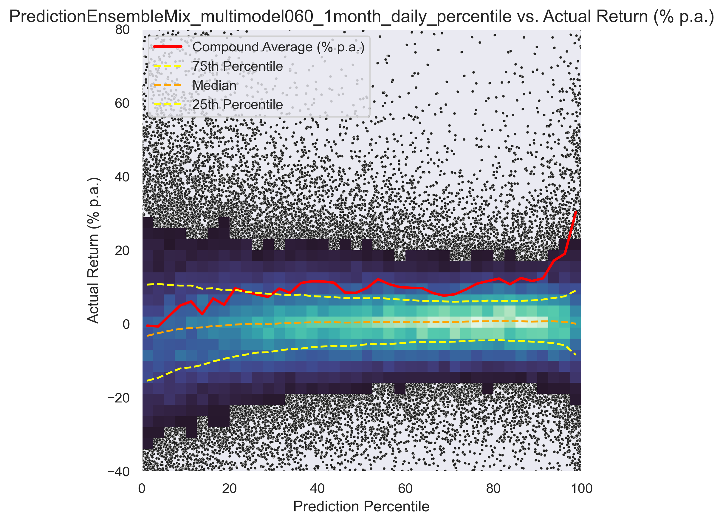
In the following graph, return (y-axis) vs. model recommendation (x-axis) for different trading models can be seen.

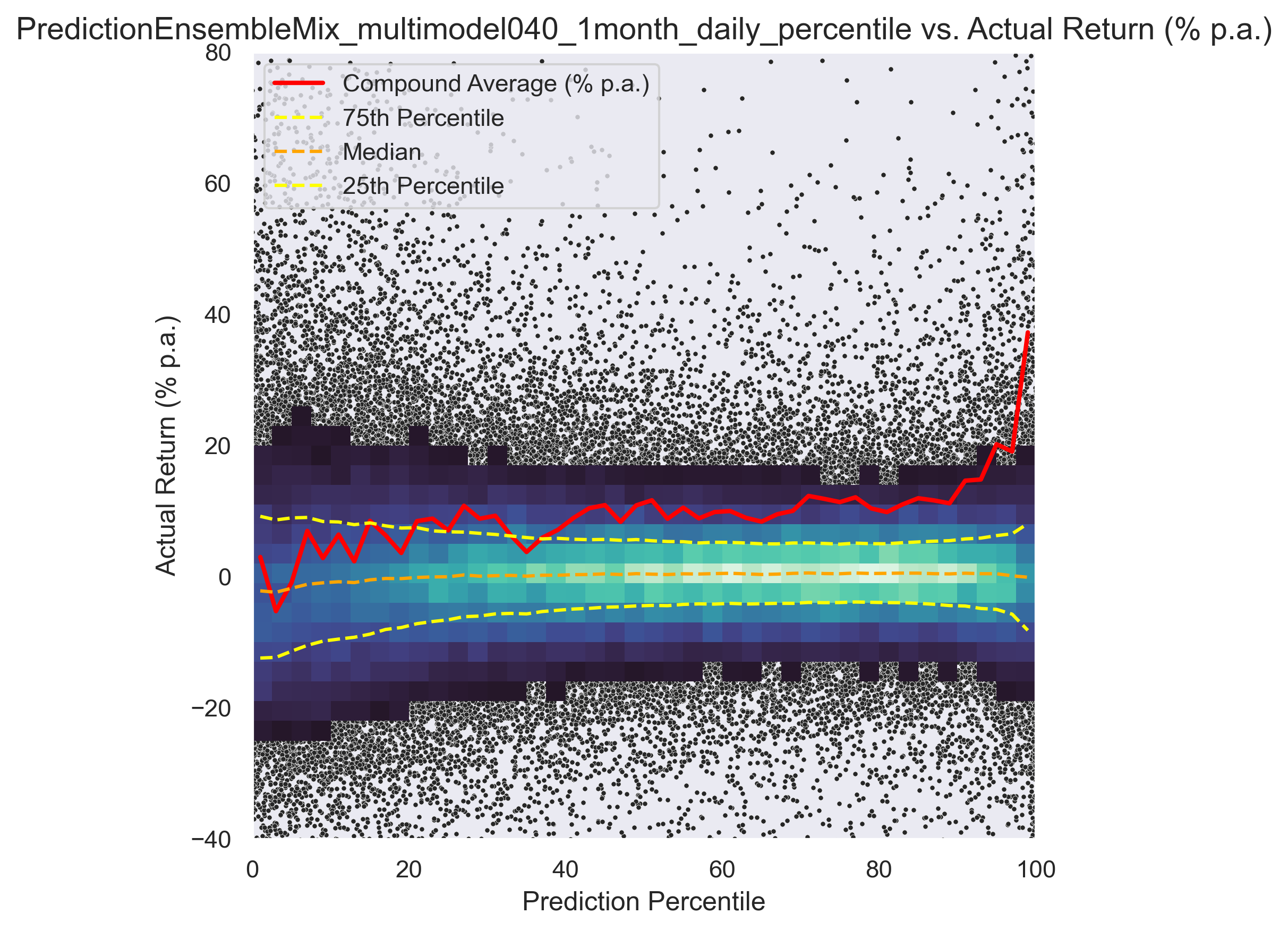
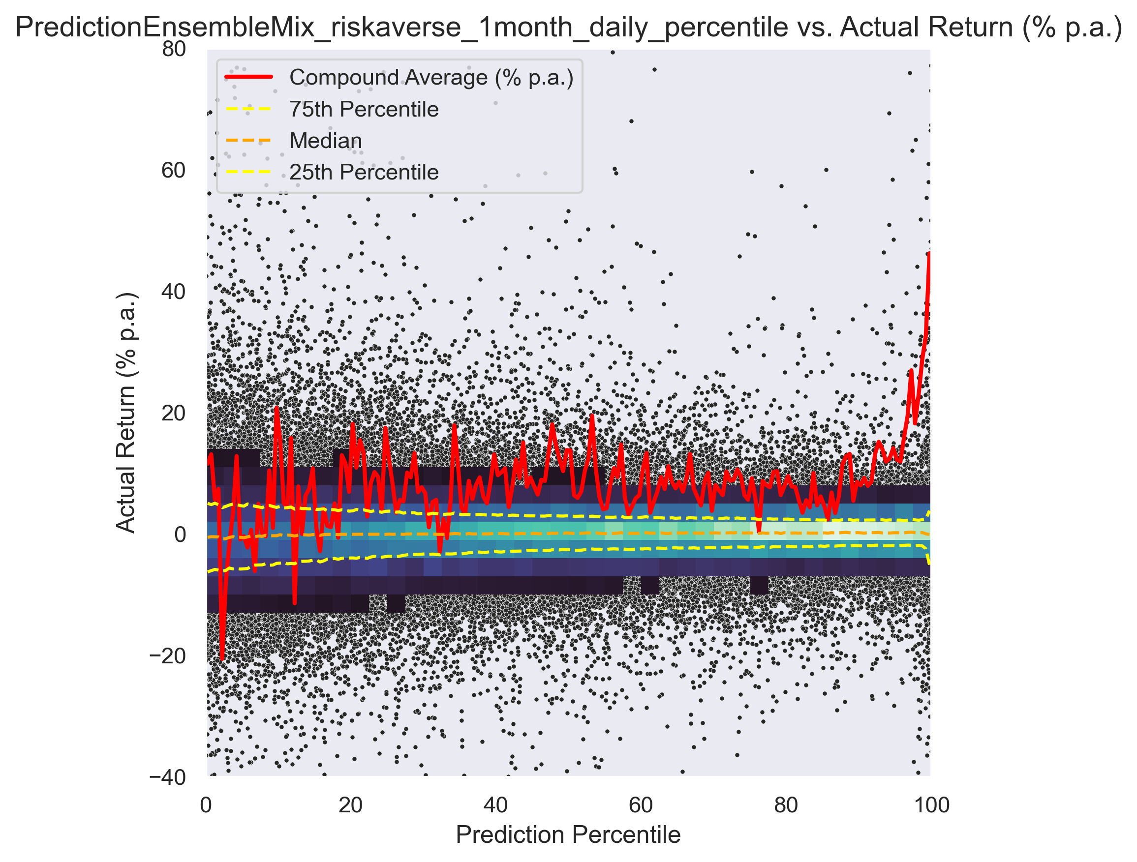
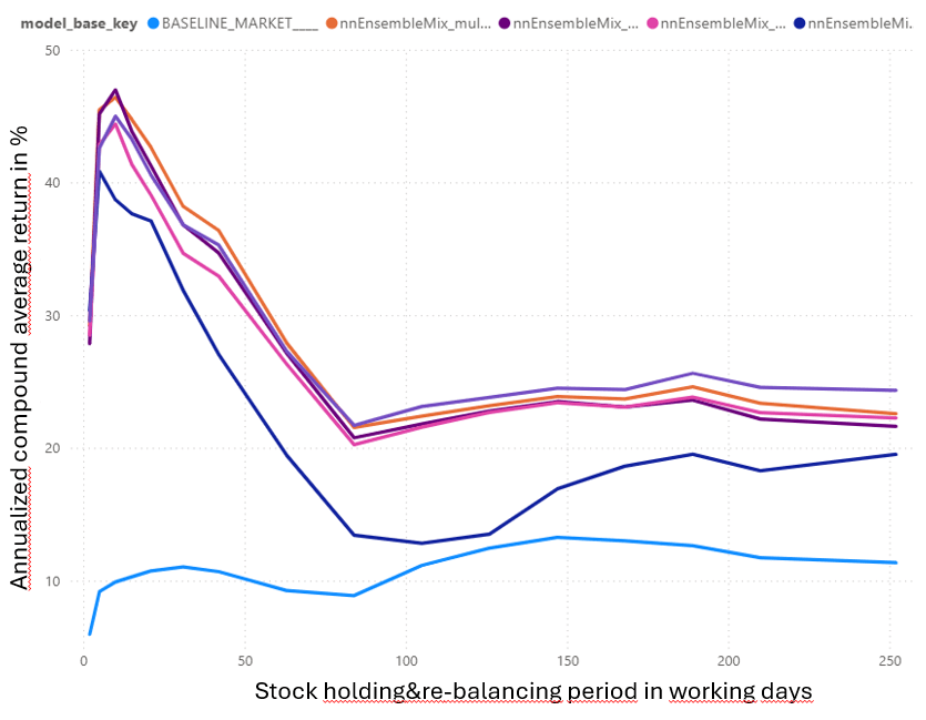
Another interesting view on the graph below. Return (excl. taxes and fees) vs. holding period